Practical 1: Multi-Layer Perceptrons

Open notebook:

Authors: Phillip Lippe

In this practical, you will get a first experience in working with images and neural networks by implementing multi-layer perceptrons (MLPs). You will experiment with different optimization and regularization strategies to get the best performance out of your model, and investigate the limitations of using MLPs for image processing. This notebook is intended to guide you through the practical and you can edit it in any place. If you prefer working with standard python scripts, feel free to convert this notebook into a python script. To open this notebook on Google Colab, use the button above. Note that you need to copy this notebook into your own Google Drive to save the notebook and trained models. Otherwise, your progress will be lost when you close the browser tab.

First of all, let’s start with importing some standard libraries:

## Standard libraries
import os
import json
import math
import numpy as np
import copy

## Imports for plotting
import matplotlib.pyplot as plt
from matplotlib import cm
%matplotlib inline
import seaborn as sns
sns.set()

## Progress bar
from tqdm.notebook import tqdm

## PyTorch
import torch
import torch.nn as nn
import torch.nn.functional as F
import torch.utils.data as data
import torch.optim as optim

## PyTorch Torchvision
import torchvision
from torchvision.datasets import CIFAR10
from torchvision import transforms

Throughout the practicals, we make use of several datasets and might want to save different models. For this, we define the two paths below. Adjust the paths as you like, but remember to keep them consistent across practicals to not download the dataset several times.

# Path to the folder where the datasets are/should be downloaded (e.g. MNIST)
DATASET_PATH = "../data"
# Path to the folder where the pretrained models are saved
CHECKPOINT_PATH = "../saved_models/practical1"
os.makedirs(CHECKPOINT_PATH, exist_ok=True)

Training deep neural networks is a stochastic process. Hence, every time you run the notebook, you naturally get different results. To obtain reproducible results, it is highly recommended to set a seed for all stochastic operations. Hence, let’s define a set_seed function below.

# Function for setting the seed
def set_seed(seed):
    np.random.seed(seed)
    torch.manual_seed(seed)
    if torch.cuda.is_available():
        torch.cuda.manual_seed(seed)
        torch.cuda.manual_seed_all(seed)
set_seed(42)

# Ensure that all operations are deterministic on GPU (if used) for reproducibility
torch.backends.cudnn.determinstic = True
torch.backends.cudnn.benchmark = False

# Fetching the device that will be used throughout this notebook
device = torch.device("cpu") if not torch.cuda.is_available() else torch.device("cuda:0")
print("Using device", device)

Using device cuda:0

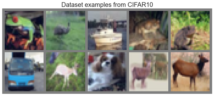
Finally, let’s start with setting up the dataset we will use in this practical: CIFAR10. CIFAR10 is a very popular dataset for computer vision on low-resolution images (32x32 pixels). The task is to classify images into one of 10 classes: airplane, automobile, bird, cat, deer, dog, frog, horse, ship, and truck. Our goal is to develop a neural network that can solve this task efficiently and accurately. To load the dataset, we can luckily make use of PyTorch’s library torchvision which provides access to many popular vision datasets and more practical functions. So, let’s load the dataset below:

# Dataset statistics for normalizing the input values to zero mean and one std
DATA_MEANS = [0.491, 0.482, 0.447]
DATA_STD = [0.247, 0.243, 0.261]

# Transformations are applied on images when we want to access them. Here, we push the images into a tensor
# and normalize the values. However, you can use more transformations, like augmentations to prevent overfitting.
# Feel free to experiment with augmentations here once you have a first running MLP, but remember to not apply
# any augmentations on the test data!
data_transforms = transforms.Compose([transforms.ToTensor(),
                                      transforms.Normalize(DATA_MEANS, DATA_STD)
                                     ])

# Loading the training dataset. We need to split it into a training and validation part
main_dataset = CIFAR10(root=DATASET_PATH, train=True, transform=data_transforms, download=True)
train_set, val_set = torch.utils.data.random_split(main_dataset, [45000, 5000], generator=torch.Generator().manual_seed(42))

# Loading the test set
test_set = CIFAR10(root=DATASET_PATH, train=False, transform=data_transforms, download=True)

# Create data loaders for later
train_loader = data.DataLoader(train_set, batch_size=128, shuffle=True, drop_last=True, pin_memory=True, num_workers=3)
val_loader = data.DataLoader(val_set, batch_size=128, shuffle=False, drop_last=False, num_workers=3)
test_loader = data.DataLoader(test_set, batch_size=128, shuffle=False, drop_last=False, num_workers=3)

Files already downloaded and verified
Files already downloaded and verified

When working with data, it is always recommend to look at the data before blaming your model for not performing well if the data was incorrectly processed. Hence, let’s plot the first 10 images of the CIFAR10 training dataset:

NUM_IMAGES = 10
images = [train_set[idx][0] for idx in range(NUM_IMAGES)]
img_grid = torchvision.utils.make_grid(torch.stack(images, dim=0), nrow=5, normalize=True, pad_value=0.5)
img_grid = img_grid.permute(1, 2, 0)

plt.figure(figsize=(12,8))
plt.title("Dataset examples from CIFAR10", fontsize=20)
plt.imshow(img_grid)
plt.axis('off')
plt.show()
plt.close()

Now we are all set. So, let’s dive into implementing our own MLP!

Part 1: Implementing the MLP

As a first step, let’s implement a simple MLP.

MLP Module

You can make use of PyTorch’s common functionalities, especially the torch.nn modules might be of help. The design choices of the MLP (e.g. the activation function) is left up to you, but for an initial setup, we recommend stacking linear layers with ReLU activation functions in between. Remember to not apply any activation function on the output.

class MLP(nn.Module):

    def __init__(self, input_size=3072, num_classes=10, hidden_sizes=[256, 128]):
        """
        Inputs:
            input_size - Size of the input images in pixels
            num_classes - Number of classes we want to predict. The output size of the MLP
                          should be num_classes.
            hidden_sizes - A list of integers specifying the hidden layer sizes in the MLP.
                           The MLP should have len(hidden_sizes)+1 linear layers.
        """
        super().__init__()
        # TODO: Create the network based on the specified hidden sizes
        raise NotImplementedError

    def forward(self, x):
        # TODO: Apply the MLP on an input
        raise NotImplementedError

# Let's test the MLP implementation
input_size = np.random.randint(low=64, high=3072)
num_classes = np.random.randint(low=5, high=20)
hidden_sizes = [np.random.randint(low=32, high=256) for _ in range(np.random.randint(low=1, high=3))]
my_mlp = MLP(input_size=input_size, num_classes=num_classes, hidden_sizes=hidden_sizes)
my_mlp.to(device)
random_input = torch.randn(32, input_size, device=device)
random_output = my_mlp(random_input)
assert random_output.shape[0] == random_input.shape[0]
assert random_output.shape[1] == num_classes

Optimizer

To gain a better insight in the training of the neural networks, let’s implement our own optimizer. First, we need to understand what an optimizer actually does. The optimizer is responsible to update the network’s parameters given the gradients. Hence, we effectively implement a function \(w^{t} = f(w^{t-1}, g^{t}, ...)\) with \(w\) being the parameters, and \(g^{t} = \nabla_{w^{(t-1)}} \mathcal{L}^{(t)}\) the gradients at time step \(t\). A common, additional parameter to this function is the learning rate, here denoted by \(\eta\). Usually, the learning rate can be seen as the “step size” of the update. A higher learning rate means that we change the weights more in the direction of the gradients, a smaller means we take shorter steps.

As most optimizers only differ in the implementation of \(f\), we can define a template for an optimizer in PyTorch below. We take as input the parameters of a model and a learning rate. The function zero_grad sets the gradients of all parameters to zero, which we have to do before calling loss.backward(). Finally, the step() function tells the optimizer to update all weights based on their gradients. The template is setup below:

class OptimizerTemplate:

    def __init__(self, params, lr):
        self.params = list(params)
        self.lr = lr

    def zero_grad(self):
        ## Set gradients of all parameters to zero
        for p in self.params:
            if p.grad is not None:
                p.grad.detach_() # For second-order optimizers important
                p.grad.zero_()

    @torch.no_grad()
    def step(self):
        ## Apply update step to all parameters
        for p in self.params:
            if p.grad is None: # We skip parameters without any gradients
                continue
            self.update_param(p)

    def update_param(self, p):
        # To be implemented in optimizer-specific classes
        raise NotImplementedError

The optimizer we are going to implement is the standard Stochastic Gradient Descent (SGD) with momentum. Plain SGD updates the parameters using the following equation:

\[\begin{split} w^{(t)} & = w^{(t-1)} - \eta \cdot g^{(t)} \end{split}\]

The concept of momentum replaces the gradient in the update by an exponential average of all past gradients including the current one, which allows for a smoother training. The gradient update with momentum becomes:

\[\begin{split}\begin{split} m^{(t)} & = \beta_1 m^{(t-1)} + (1 - \beta_1)\cdot g^{(t)}\\ w^{(t)} & = w^{(t-1)} - \eta \cdot m^{(t)}\\ \end{split}\end{split}\]

Let’s implement the optimizer below:

class SGDMomentum(OptimizerTemplate):

    def __init__(self, params, lr, momentum=0.9):
        super().__init__(params, lr)
        self.momentum = momentum # Corresponds to beta_1 in the equation above
        self.param_momentum = {p: torch.zeros_like(p.data) for p in self.params} # Dict to store m_t

    def update_param(self, p):
        # TODO: Implement the gradient update
        raise NotImplementedError

To verify that our optimizer is working, let’s create a challenging surface over two parameter dimensions which we want to optimize to find the optimum:

def pathological_curve_loss(w1, w2):
    # Example of a pathological curvature. There are many more possible, feel free to experiment here!
    x1_loss = torch.tanh(w1)**2 + 0.01 * torch.abs(w1)
    x2_loss = torch.sigmoid(w2)
    return x1_loss + x2_loss

def plot_curve(curve_fn, x_range=(-5,5), y_range=(-5,5), plot_3d=False, cmap=cm.viridis, title="Pathological curvature"):
    fig = plt.figure(figsize=(6, 6))
    ax = fig.gca(projection='3d') if plot_3d else fig.gca()

    x = torch.arange(x_range[0], x_range[1], (x_range[1]-x_range[0])/100.)
    y = torch.arange(y_range[0], y_range[1], (y_range[1]-y_range[0])/100.)
    x, y = torch.meshgrid([x,y], indexing='ij')
    z = curve_fn(x, y)
    x, y, z = x.numpy(), y.numpy(), z.numpy()

    if plot_3d:
        ax.plot_surface(x, y, z, cmap=cmap, linewidth=1, color="#000", antialiased=False)
        ax.set_zlabel("loss")
    else:
        ax.imshow(z.T[::-1], cmap=cmap, extent=(x_range[0], x_range[1], y_range[0], y_range[1]))
    plt.title(title)
    ax.set_xlabel(r"$w_1$")
    ax.set_ylabel(r"$w_2$")
    plt.tight_layout()
    return ax

sns.reset_orig()
_ = plot_curve(pathological_curve_loss, plot_3d=True)
plt.show()

In terms of optimization, you can image that \(w_1\) and \(w_2\) are weight parameters, and the curvature represents the loss surface over the space of \(w_1\) and \(w_2\). Note that in typical networks, we have many, many more parameters than two, and such curvatures can occur in multi-dimensional spaces as well.

Ideally, our optimization algorithm would find the center of the ravine and focuses on optimizing the parameters towards the direction of \(w_2\). However, if we encounter a point along the ridges, the gradient is much greater in \(w_1\) than \(w_2\), and we might end up jumping from one side to the other. Due to the large gradients, we would have to reduce our learning rate slowing down learning significantly.

To test our algorithms, we can implement a simple function to train two parameters on such a surface:

def train_curve(optimizer_func, curve_func=pathological_curve_loss, num_updates=100, init=[5,5]):
    """
    Inputs:
        optimizer_func - Constructor of the optimizer to use. Should only take a parameter list
        curve_func - Loss function (e.g. pathological curvature)
        num_updates - Number of updates/steps to take when optimizing
        init - Initial values of parameters. Must be a list/tuple with two elements representing w_1 and w_2
    Outputs:
        Numpy array of shape [num_updates, 3] with [t,:2] being the parameter values at step t, and [t,2] the loss at t.
    """
    weights = nn.Parameter(torch.FloatTensor(init), requires_grad=True)
    optimizer = optimizer_func([weights])

    list_points = []
    for _ in range(num_updates):
        # TODO: Determine the loss for the current weights, save the weights and loss, perform backpropagation
        raise NotImplementedError

    points = torch.stack(list_points, dim=0).numpy()
    return points

Next, let’s apply the optimizer on our curvature. Note that we set a much higher learning rate for the optimization algorithms as you would in a standard neural network. This is because we only have 2 parameters instead of tens of thousands or even millions.

SGDMom_points = train_curve(lambda params: SGDMomentum(params, lr=10, momentum=0.9))

To understand best how the different algorithms worked, we visualize the update step as a line plot through the loss surface. We will stick with a 2D representation for readability.

all_points = SGDMom_points
ax = plot_curve(pathological_curve_loss,
                x_range=(-np.absolute(all_points[:,0]).max(), np.absolute(all_points[:,0]).max()),
                y_range=(all_points[:,1].min(), all_points[:,1].max()),
                plot_3d=False)
ax.plot(SGDMom_points[:,0], SGDMom_points[:,1], color="red", marker="o", zorder=2, label="SGDMom")
plt.legend()
plt.show()

If the implementation is correct, you should see that the optimizer indeed reaches a point of very low \(w_2\) (\(w_2 < -7.5\)) and \(w_1\approx 0\). If not, go back to your optimizer implementation and check what could go wrong.

Training and validation function

Now that we the MLP ready, the optimizer implemented, and the dataset loaded, we can look at implementing our own training function. The form of the training function is left mostly up to you, but we recommend that you test the model on the validation function after every 5 epochs, and save the best model. We provide a rough template below.

def train_model(model, optimizer, train_data_loader, val_data_loader, num_epochs=25, model_name="MyMLP"):
    # Set model to train mode
    model.to(device)
    best_val_acc = -1.0

    # Training loop
    for epoch in range(1, num_epochs+1):
        model.train()
        for imgs, labels in train_data_loader:
            # TODO: Implement training loop with training on classification
            raise NotImplementedError

        if epoch % 5 == 0:
            # TODO: Evaluate the model and save if best
            raise NotImplementedError

    # Load best model after training
    load_model(model, model_name)

@torch.no_grad()
def test_model(model, data_loader):
    # TODO: Test model and return accuracy
    raise NotImplementedError

def save_model(model, model_name):
    # TODO: Save the parameters of the model
    raise NotImplementedError

def load_model(model, model_name):
    # TODO: Load the parameters of the model
    raise NotImplementedError

# TODO: Create model, optimizer, and start training
raise NotImplementedError

# TODO: Test best model on test set
raise NotImplementedError

It is expected that you reach with the default configurations a validation and test accuracy of \(\sim52-53\%\) . If you have reached this performance, we can consider this task as completed!

Part 2: Improving your MLP

Now that we have a basic MLP, let’s try to improve over this default performance! Your task is to think about ways to maximize the performance of your MLP. Possible suggestions you can look at include:

• Do data augmentations help the model to generalize?

• Can regularization techniques (dropout, weight decay, etc.) help?

• Do deeper models perform better? Or is it better to have wide networks?

• Can normalization techniques (BatchNorm, LayerNorm, etc.) help?

Your task is to improve your model to reach at least 56% on the test set! But can you get even above this? Consider this as a challenge!

For this implementation, you can directly edit your model above. In your report, list the changes that you have made and discuss what affect they have. Further, repeat the experiment for at least 3 seeds to report stable improvements.

# TODO: Improve the model
raise NotImplementedError

Part 3: Investigating the limitations

Now that we have seen how we can optimize our MLP, it is good to investigate the limitations of the model as well. Images have a natural grid structure where close-by pixels are strongly related. Does the MLP make use of this structure? To investigate this question, we will run two experiments:

• Create a shuffle of pixels at the beginning of the training, and use the same shuffle throughout the training and validation.

• At each training and validation step, sample a new shuffle of pixels.

It is up to you whether you perform this investigation on the original plain MLP version or your optimized one. Implement a corresponding train and test function that support both variants of shuffling, and train two models.

# TODO: Create a training and test function that supports the shuffling of pixels, both fixed and newly generated for each batch
raise NotImplementedError

# TODO: Create model, optimizer, and start training on fixed shuffling of pixels
raise NotImplementedError

# TODO: Create model, optimizer, and start training on a new shuffling of pixels per batch/image
raise NotImplementedError

What results do you observe? What does this tell us about the MLP being aware of the image structure? Add your results and observations to your report.

Conclusion

You have reached the end of the practical, congratulations! Now, you should have a good idea of what it means to train a MLP, how we can use neural networks to perform image classification, and what tricks there are to improve a networks performance. In the next practicals, we will look at more advanced network structures beyond MLPs.